Convolutional Neural Network for Handwritten Digits Recognition
 LeNet-5 Architecture
In this post, we will build, train and optimize in TensorFlow one of the simplest Convolutional Neural Networks, LeNet-5, proposed by Yann LeCun, Leon Bottou, Yosuha Bengio and Patrick Haffner in 1998 (for more details, check the paper “Gradient-Based Learning Applied to Document Recognition”, Y.LeCun et al.).
import tensorflow as tf
import numpy as np
from tensorflow.examples.tutorials.mnist import input_data

mnist = input_data.read_data_sets("MNIST_data/", one_hot=True)
X_train, y_train           = mnist.train.images, mnist.train.labels
X_validation, y_validation = mnist.validation.images, mnist.validation.labels
X_test, y_test             = mnist.test.images, mnist.test.labels

print("Image Shape: {}".format(X_train[0].shape))
print("Training Set:   {} samples".format(len(X_train)))
print("Validation Set: {} samples".format(len(X_validation)))
print("Test Set:       {} samples".format(len(X_test)))

epsilon = 1e-10 # this is a parameter you will use later
Image Shape: (784,)
Training Set:   55000 samples
Validation Set: 5000 samples
Test Set:       10000 samples
Introduction to Tensorflow 101
TensorFlow Static Graph
The entire purpose of Tensorflow is to have a so-called computational graph that can be executed much more efficiently than if the same calculations were to be performed directly in Python. TensorFlow can be more efficient than NumPy because TensorFlow knows the entire computation graph that must be executed, while NumPy only knows the computation of a single mathematical operation at a time.
TensorFlow can also automatically calculate the gradients that are needed to optimize the variables of the graph so as to make the model perform better. This is because the graph is a combination of simple mathematical expressions so the gradient of the entire graph can be calculated using the chain-rule for derivatives.
TensorFlow can also take advantage of multi-core CPUs as well as GPUs - and Google has even built special hardware accelerators just for TensorFlow which are called TPUs (Tensor Processing Units) that are even faster than GPUs.
A TensorFlow graph consists of the following parts which will be detailed below:
- Placeholder variables used to feed input into the graph.
- Model variables that are going to be optimized so as to make the model perform better.
- The model which is essentially just a mathematical function that calculates some output given the input in the placeholder variables and the model variables.
- A cost measure that can be used to guide the optimization of the variables.
- An optimization method which updates the variables of the model.
In addition, the TensorFlow graph may also contain various debugging statements e.g. for logging data to be displayed using TensorBoard.
Placeholder variables
Placeholder variables serve as the input to the graph that we may change each time we execute the graph. We call this feeding the placeholder variables and it is demonstrated further below.
First we define the placeholder variable for the input images. This allows us to change the images that are input to the TensorFlow graph. This is a so-called tensor, which just means that it is a multi-dimensional vector or matrix. The data-type is set to float32 and the shape is set to [None, img_size_flat], where None means that the tensor may hold an arbitrary number of images with each image being a vector of length img_size_flat (in our case it’s 784).
x = tf.placeholder(tf.float32, [None, 784], name='inputs')
print(x)
Tensor("inputs:0", shape=(?, 784), dtype=float32)
Next we have the placeholder variable for the true labels associated with the images that were input in the placeholder variable x.
The shape of this placeholder variable is [None, num_classes] which means it may hold an arbitrary number of labels and each label is a vector of length num_classes which is 10 in this case.
y_true = tf.placeholder(tf.float32, [None, 10], name='labels')
print(y_true)
Tensor("labels:0", shape=(?, 10), dtype=float32)
Finally we have the tensor variable for the true class of each image in the placeholder variable x. These are integers and the dimensionality of this placeholder variable is set to [None] which means the placeholder variable is a one-dimensional vector of arbitrary length.
y_true_cls = tf.argmax(y_true, 1)
Variables to be optimized
Apart from the placeholder variables that were defined above and which serve as feeding input data into the model, there are also some model variables that must be changed by TensorFlow so as to make the model perform better on the training data.
The first variable that must be optimized is called weights and is defined here as a TensorFlow variable that must be initialized with zeros and whose shape is [img_size_flat, num_classes], so it is a 2-dimensional tensor (or matrix) with img_size_flat rows and num_classes columns.
weights = tf.Variable(tf.zeros([784, 10]), name='weights')
print(weights)
<tf.Variable 'weights:0' shape=(784, 10) dtype=float32_ref>
The second variable that must be optimized is called biases and is defined as a 1-dimensional tensor (or vector) of length num_classes.
biases = tf.Variable(tf.zeros([10]), name='bias')
print(biases)
<tf.Variable 'bias:0' shape=(10,) dtype=float32_ref>
Model
This simple mathematical model multiplies the images in the placeholder variable x with the weights and then adds the biases.
The result is a matrix of shape [num_images, num_classes] because x has shape [num_images, img_size_flat] and weights has shape [img_size_flat, num_classes], so the multiplication of those two matrices is a matrix with shape [num_images, num_classes] and then the biases vector is added to each row of that matrix.
Note that the name logits is typical TensorFlow terminology, but other people may call the variable something else.
Now logits is a matrix with num_images rows and num_classes columns, where the element of the $i$‘th row and $j$‘th column is an estimate of how likely the $i$‘th input image is to be of the $j$‘th class.
However, these estimates are a bit rough and difficult to interpret because the numbers may be very small or large, so we want to normalize them so that each row of the logits matrix sums to one, and each element is limited between zero and one. This is calculated using the so-called softmax function and the result is stored in y_pred.
The predicted class can be calculated from the y_pred matrix by taking the index of the largest element in each row.
with tf.name_scope('model'):
    logits = tf.matmul(x, weights) + biases
    y_pred = tf.nn.softmax(logits)
    y_pred_cls = tf.argmax(y_pred, axis=1)
Cost-function to be optimized
To make the model better at classifying the input images, we must somehow change the variables for weights and biases. To do this we first need to know how well the model currently performs by comparing the predicted output of the model y_pred to the desired output y_true.
The cross-entropy is a performance measure used in classification. The cross-entropy is a continuous function that is always positive and if the predicted output of the model exactly matches the desired output then the cross-entropy equals zero. The goal of optimization is therefore to minimize the cross-entropy so it gets as close to zero as possible by changing the weights and biases of the model.
TensorFlow has a built-in function for calculating the cross-entropy. Note that it uses the values of the logits because it also calculates the softmax internally.
After that, we have the cross-entropy for each of the image classifications so we have a measure of how well the model performs on each image individually. But in order to use the cross-entropy to guide the optimization of the model’s variables we need a single scalar value, so we simply take the average of the cross-entropy for all the image classifications.
with tf.name_scope('loss'):
    cross_entropy = tf.nn.softmax_cross_entropy_with_logits_v2(logits=logits,
                                                               labels=y_true)
    loss = tf.reduce_mean(cross_entropy)
Optimization
Now that we have a cost measure that must be minimized, we can then create an optimizer. In this case it is the basic form of Gradient Descent where the step-size is set to 0.01.
Note that optimization is not performed at this point. In fact, nothing is calculated at all, we just add the optimizer-object to the TensorFlow graph for later execution.
learning_rate = 0.01
with tf.name_scope('optim'):
    optimizer = tf.train.GradientDescentOptimizer(learning_rate)
    opt_step = optimizer.minimize(loss)
Performance
We need a few more performance measures to display the progress to the user.
This is a vector of booleans whether the predicted class equals the true class of each image.
This calculates the classification accuracy by first type-casting the vector of booleans to floats, so that False becomes 0 and True becomes 1, and then calculating the average of these numbers.
with tf.name_scope('accuracy'):
    correct_prediction = tf.equal(y_pred_cls, y_true_cls)
    accuracy = tf.reduce_mean(tf.cast(correct_prediction, tf.float32))
TensorFlow Session
Once the TensorFlow graph has been created, we have to create a TensorFlow session which is used to execute the graph.
session = tf.Session()
Initialize variables
The variables for weights and biases must be initialized before we start optimizing them.
init_op = tf.global_variables_initializer()
session.run(init_op)
Setup the TensorBoard
Tensorboard is shipped with TensorFlow and it’s a tool that allows to plot metrics, debug the graph, and much more.
def next_path(path_pattern):
    import os
    i = 1
    while os.path.exists(path_pattern % i):
        i = i * 2
    a, b = (i / 2, i)
    while a + 1 < b:
        c = (a + b) / 2
        a, b = (c, b) if os.path.exists(path_pattern % c) else (a, c)
    directory = path_pattern % b
    return directory


writer = tf.summary.FileWriter(next_path('logs/run_%02d'))
tf.summary.scalar("Loss", loss)
tf.summary.scalar("Accuracy", accuracy)
merged_summary_op = tf.summary.merge_all()
Time to learn
Now that everything is defined, we can move to running the optimization. There are 55.000 images in the training-set. It takes a long time to calculate the gradient of the model using all these images. We therefore use Stochastic Gradient Descent which only uses a small batch of images in each iteration of the optimizer.
batch_size = 100
Function for performing a number of optimization iterations so as to gradually improve the weights and biases of the model. In each iteration, a new batch of data is selected from the training-set and then TensorFlow executes the optimizer using those training samples.
Let’s define a couple of functions that will be usefull later.
def optimize(epochs):
    # Go through the traning dataset `epochs` times
    for e in range(epochs):

        num_of_batches = int(mnist.train.num_examples/batch_size)

        # We save also the loss across all the batches of data for
        # presentation purpose
        avg_loss = 0.

        # Loop over all batches
        for i in range(num_of_batches):
            # Get a batch of training examples (shuffle every epoch).
            # x_batch now holds a batch of images and
            # y_true_batch are the true labels for those images.
            x_batch, y_true_batch = mnist.train.next_batch(batch_size, shuffle=(i==0))

            # Put the batch into a dict with the proper names
            # for placeholder variables in the TensorFlow graph.
            # Note that the placeholder for y_true_cls is not set
            # because it is not used during training.
            feed_dict_train = {x: x_batch,
                               y_true: y_true_batch}

            # Run the optimizer using this batch of training data.
            # TensorFlow assigns the variables in feed_dict_train
            # to the placeholder variables and then runs the optimizer.
            session.run(opt_step, feed_dict=feed_dict_train)

            # Similarly, get the loss and accuracy metrics on the batch of data
            batch_loss, summary = session.run([loss, merged_summary_op], feed_dict=feed_dict_train)

            # Write logs at every iteration
            writer.add_summary(summary, e * num_of_batches + i)

            # Compute average loss
            avg_loss += batch_loss / num_of_batches

        print("Epoch: ", '%02d' % (e + 1), "  =====> Loss =", "{:.6f}".format(avg_loss))

def print_accuracy():
    feed_dict_test = {x: mnist.test.images,
                  y_true: mnist.test.labels}

    # Use TensorFlow to compute the accuracy.
    # We are also going to save some metric like memory usage and computation time
    run_options = tf.RunOptions(trace_level=tf.RunOptions.FULL_TRACE)
    run_metadata = tf.RunMetadata()
    acc = session.run(accuracy, feed_dict=feed_dict_test, options=run_options, run_metadata=run_metadata)
    try:
        writer.add_run_metadata(run_metadata, 'inference')
    except ValueError:
        pass
    writer.flush()
    # Print the accuracy.
    print("Accuracy on test-set: {0:.1%}".format(acc))
Let’s add the graph to TensorBoard for easy debugging
writer.add_graph(tf.get_default_graph())
Performance before any optimization
The accuracy on the test-set is 9.8%. This is because the model has only been initialized and not optimized at all, so it always predicts that the image shows a zero digit and it turns out that 9.8% of the images in the test-set happens to be zero digits.
print_accuracy()
Accuracy on test-set: 9.8%
Now we can train the model for 50 epochs and print the accuracy.
optimize(50)
print_accuracy()
Epoch:  01   =====> Loss = 1.177169
.
.
.
Epoch:  50   =====> Loss = 0.303337
Accuracy on test-set: 91.9%
Using Tensorboard, we can now visualize the created graph, giving you an overview of your architecture and how all of the major components are connected. We can also see and analyse the learning curves.
We can launch TensorBoard by opening a Terminal and running the command line tensorboard --logdir logs
LeNet5
We are now familar with TensorFlow and TensorBoard. In this section, we are going to build, train and test the baseline LeNet-5 model for the MNIST digits recognition problem.
Then, we will make some optimizations to get more than 99% of accuracy.
For more informations, here is a list of results: http://rodrigob.github.io/are_we_there_yet/build/classification_datasets_results.html

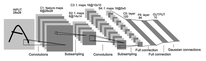
The LeNet architecture takes a 28x28xC image as input, where C is the number of color channels. Since MNIST images are grayscale, C is 1 in this case.
Layer 1 - Convolution (5x5): The output shape should be 28x28x6. Activation: ReLU. MaxPooling: The output shape should be 14x14x6.
Layer 2 - Convolution (5x5): The output shape should be 10x10x16. Activation: ReLU. MaxPooling: The output shape should be 5x5x16.
Flatten: Flatten the output shape of the final pooling layer such that it’s 1D instead of 3D. You may need to use tf.reshape.
Layer 3 - Fully Connected: This should have 120 outputs. Activation: ReLU.
Layer 4 - Fully Connected: This should have 84 outputs. Activation: ReLU.
Layer 5 - Fully Connected: This should have 10 outputs. Activation: softmax.
Implementing the Neural Network architecture described above. For that, we will use classes and functions from https://www.tensorflow.org/api_docs/python/tf/nn.
# Functions for weigths and bias initilization
def weight_variable(shape, name):
    initial = tf.truncated_normal(shape, stddev=0.1)
    return tf.Variable(initial, name=name)

def bias_variable(shape, name):
    initial = tf.constant(0., shape=shape)
    return tf.Variable(initial, name=name)
def build_lenet5(x):
    with tf.name_scope("reshape"):
        image = tf.reshape(x, [-1, 28, 28, 1]) # [None, 28, 28, 1]

    with tf.name_scope("lenet5"):
        with tf.name_scope("layer1"):
            weights1 = weight_variable([5,5,1,6],"weights1")
            bias1 = bias_variable([6],"bias1")
            conv1 = tf.nn.conv2d(image,weights1, strides = [1,1,1,1], padding = 'SAME') + bias1
            conv1 = tf.nn.relu(conv1)
            maxpool1 = tf.nn.max_pool(conv1, ksize= [1,2,2,1], strides= [1,2,2,1] , padding = 'VALID')

        with tf.name_scope("layer2"):
            weights2 = weight_variable([5,5,6,16],"weights2")
            bias2 = bias_variable([16],"bias2")
            conv2 = tf.nn.conv2d (maxpool1, weights2, strides= [1,1,1,1], padding = 'VALID') + bias2
            conv2 = tf.nn.relu(conv2)
            maxpool2 = tf.nn.max_pool(conv2,ksize= [1,2,2,1], strides= [1,2,2,1] , padding = 'VALID')


        with tf.name_scope("flatten"):
            flat = tf.contrib.layers.flatten(maxpool2)

        with tf.name_scope("layer3"):
            weights3 = weight_variable((400,120),"weights3")
            bias3 = bias_variable([120],"bias3")
            res3 = tf.matmul(flat,weights3) + bias3
            res3 = tf.nn.relu(res3)

        with tf.name_scope("layer4"):
            weights4 = weight_variable((120,84),"weights4")
            bias4 = bias_variable([84],"bias4")
            res4 = tf.matmul(res3,weights4) + bias4
            res4 = tf.nn.relu(res4)

        with tf.name_scope("layer5"):
            weights5 = weight_variable((84,10),"weights5")
            bias5 = bias_variable([10],"bias5")
            res5 = tf.matmul(res4,weights5) + bias5
            out = tf.nn.softmax(res5)

    return res5, out
The number of parameters of this model
| layer | weights | biases | total |
|---|---|---|---|
| $1$ | $5\times5\times1\times6=150$ | $6$ | $156$ |
| $2$ | $5\times5\times6\times16=2400$ | $16$ | $2416$ |
| $3$ | $400\times120=48000$ | $120$ | $48120$ |
| $4$ | $120\times84=10080$ | $84$ | $10164$ |
| $5$ | $84\times10=840$ | $10$ | $850$ |
| Total | $61706$ |
Defining the model, its accuracy and the loss function according to the following parameters:
 Learning rate: 0.001
 Loss Fucntion: Cross-entropy
 Optimizer: tf.train.GradientDescentOptimizer
 Number of epochs: 40
 Batch size: 128
# Parameters
learning_rate = 0.001
batch_size = 128
epochs = 40
tf.reset_default_graph() # reset the default graph before defining a new model

# Model, loss function and accuracy
x = tf.placeholder(tf.float32, [None, 784], name='inputs')
y_true = tf.placeholder(tf.float32, [None, 10], name='labels')
y_true_cls = tf.argmax(y_true, 1)

with tf.name_scope('model'):
    logits, y_pred = build_lenet5(x)
    y_pred_cls = tf.argmax(y_pred, 1)

with tf.name_scope('loss'):
    cross_entropy = tf.nn.softmax_cross_entropy_with_logits_v2(logits=logits, labels=y_true)
    loss = tf.reduce_mean(cross_entropy)

with tf.name_scope('optim'):
    optimizer = tf.train.GradientDescentOptimizer(learning_rate)
    opt_step = optimizer.minimize(loss)

with tf.name_scope('accuracy'):
    correct_prediction = tf.equal(y_pred_cls, y_true_cls)
    accuracy = tf.reduce_mean(tf.cast(correct_prediction, tf.float32))
Implementing training pipeline and running the training data through it to train the model.
- Shuffling the training set before each epoch.
- Printing the loss per mini batch and the training/validation accuracy per epoch.
- Saving the model after training.
- Printing after training the final testing accuracy .
def train(init_op, session, epochs, batch_size, loss, merged_summary_op):
    session.run(init_op)
    writer = tf.summary.FileWriter(next_path('logs/lenet5/run_%02d'))
    writer.add_graph(tf.get_default_graph())

    # metrics = {'loss':[], 'val_acc':[], 'test_acc':[]}
    feed_dict_test = {x: mnist.test.images, y_true: mnist.test.labels}
    feed_dict_val = {x: mnist.validation.images, y_true: mnist.validation.labels}

    # Go through the traning dataset `epochs` times
    for e in range(epochs):

        num_of_batches = int(mnist.train.num_examples/batch_size)

        # We save also the loss across all the batches of data for
        # presentation purpose
        avg_loss = 0.

        # Loop over all batches
        for i in range(num_of_batches):
            # Get a batch of training examples (shuffle every epoch).
            # x_batch now holds a batch of images and
            # y_true_batch are the true labels for those images.
            x_batch, y_true_batch = mnist.train.next_batch(batch_size, shuffle=(i==0))

            # Put the batch into a dict with the proper names
            # for placeholder variables in the TensorFlow graph.
            # Note that the placeholder for y_true_cls is not set
            # because it is not used during training.
            feed_dict_train = {x: x_batch,
                               y_true: y_true_batch}

            # Run the optimizer using this batch of training data.
            # TensorFlow assigns the variables in feed_dict_train
            # to the placeholder variables and then runs the optimizer.
            session.run(opt_step, feed_dict=feed_dict_train)

            # Similarly, get the loss and accuracy metrics on the batch of data
            batch_loss, summary = session.run([loss, merged_summary_op], feed_dict=feed_dict_train)
            # Write logs at every iteration
            writer.add_summary(summary, e * num_of_batches + i)

            # Compute average loss
            avg_loss += batch_loss / num_of_batches
        val_acc = accuracy.eval(session=session, feed_dict=feed_dict_val)
        test_acc = accuracy.eval(session=session, feed_dict=feed_dict_test)
        #metrics['loss'].append(avg_loss)
        #metrics['val_acc'].append(val_acc)
        #metrics['test_acc'].append(test_acc)
        if (e+1)%10==0:
            print("Epoch: ", '%02d' % (e + 1))
            print("=====> Loss = {:.6f}".format(avg_loss))
            print("=====> Validation Acc: {0:.1%}".format(val_acc))
            print("=====> Test Acc: {0:.1%}".format(test_acc),"\n")
session = tf.Session()
init_op = tf.global_variables_initializer()

tf.summary.scalar("Loss", loss)
tf.summary.scalar("Accuracy", accuracy)
merged_summary_op = tf.summary.merge_all()

with tf.Session() as session:
    train(init_op, session, epochs, batch_size, loss, merged_summary_op)
Epoch:  10
=====> Loss = 0.587242
=====> Validation Acc: 86.1%
=====> Test Acc: 86.6%

Epoch:  20
=====> Loss = 0.256747
=====> Validation Acc: 92.4%
=====> Test Acc: 92.9%

Epoch:  30
=====> Loss = 0.191738
=====> Validation Acc: 94.6%
=====> Test Acc: 94.6%

Epoch:  40
=====> Loss = 0.154950
=====> Validation Acc: 95.6%
=====> Test Acc: 95.7%
Using TensorBoard to visualise and save loss and accuracy curves.


Improve the LeNET 5 Optimization
- Retraining the network with AdamOptimizer:
| Optimizer | Gradient Descent | AdamOptimizer |
|---|---|---|
| Testing Accuracy | $95.7%$ | $99.0%$ |
| Training Time | $819 s$ | $806 s$ |
- Comparing optimizers:
Using the same dataset to train and test both models, we can see that the model based on the AdamOptimizer performs better than the Gradient one. In fact, using the AdamOptimizer, the testing accuracy reaches $99.0%$ versus an accuray equals to $95.7%$ for the Gradient Descent model.
However, the training time of the AdamOptimizer model is a bit longer ($13s$ more) than the Gradient Descent one. Which is a great tradoff between accuracy and training time.

tf.reset_default_graph() # reset the default graph before defining a new model

# Model, loss function and accuracy
x = tf.placeholder(tf.float32, [None, 784], name='inputs')
y_true = tf.placeholder(tf.float32, [None, 10], name='labels')
y_true_cls = tf.argmax(y_true, 1)

with tf.name_scope('model'):
    logits, y_pred = build_lenet5(x)
    y_pred_cls = tf.argmax(y_pred, 1)

with tf.name_scope('loss'):
    cross_entropy = tf.nn.softmax_cross_entropy_with_logits_v2(logits=logits,
                                                               labels=y_true)
    loss = tf.reduce_mean(cross_entropy)

with tf.name_scope('optim'):
    optimizer = tf.train.AdamOptimizer(learning_rate)
    opt_step = optimizer.minimize(loss)

with tf.name_scope('accuracy'):
    correct_prediction = tf.equal(y_pred_cls, y_true_cls)
    accuracy = tf.reduce_mean(tf.cast(correct_prediction, tf.float32))
session = tf.Session()
init_op = tf.global_variables_initializer()

tf.summary.scalar("Loss", loss)
tf.summary.scalar("Accuracy", accuracy)
merged_summary_op = tf.summary.merge_all()

with tf.Session() as session:
    train(init_op, session, epochs, batch_size, loss, merged_summary_op)
Epoch:  10
=====> Loss = 0.014764
=====> Validation Acc: 98.6%
=====> Test Acc: 98.4%

Epoch:  20
=====> Loss = 0.004381
=====> Validation Acc: 98.8%
=====> Test Acc: 98.7%

Epoch:  30
=====> Loss = 0.001941
=====> Validation Acc: 98.9%
=====> Test Acc: 98.8%

Epoch:  40
=====> Loss = 0.000549
=====> Validation Acc: 99.0%
=====> Test Acc: 99.0%
Trying to add dropout (keep_prob = 0.75) before the first fully connected layer. We will use tf.nn.dropout for that purpose.
Accuracy achieved on testing data:
Training Accuracy: $98.8%$
The dropout regularization method is used to avoid model overfitting. In our case, we didn’t face this problem because the training accuracy is as high as the validation accuracy. That’s why the performance of the model didn’t improve after using dropout (the accuracy decreased: $98.8%$).
def build_lenet5_dropout(x):
    with tf.name_scope("reshape"):
        image = tf.reshape(x, [-1, 28, 28, 1]) # [None, 28, 28, 1]

    with tf.name_scope("lenet5"):
        with tf.name_scope("layer1"):
            weights1 = weight_variable([5,5,1,6],"weights1")
            bias1 = bias_variable([6],"bias1")
            conv1 = tf.nn.conv2d(image,weights1, strides = [1,1,1,1], padding = 'SAME') + bias1
            conv1 = tf.nn.relu(conv1)
            maxpool1 = tf.nn.max_pool(conv1, ksize= [1,2,2,1], strides= [1,2,2,1] , padding = 'VALID')

        with tf.name_scope("layer2"):
            weights2 = weight_variable([5,5,6,16],"weights2")
            bias2 = bias_variable([16],"bias2")
            conv2 = tf.nn.conv2d (maxpool1, weights2, strides= [1,1,1,1], padding = 'VALID') + bias2
            conv2 = tf.nn.relu(conv2)
            maxpool2 = tf.nn.max_pool(conv2,ksize= [1,2,2,1], strides= [1,2,2,1] , padding = 'VALID')


        with tf.name_scope("flatten"):
            flat = tf.contrib.layers.flatten(maxpool2)

        with tf.name_scope("dropout"):
            dropout = tf.nn.dropout(flat, keep_prob=0.75)

        with tf.name_scope("layer3"):
            weights3 = weight_variable([400,120],"weights3")
            bias3 = bias_variable([120],"bias3")
            res3 = tf.matmul(dropout,weights3) + bias3
            res3 = tf.nn.relu(res3)

        with tf.name_scope("layer4"):
            weights4 = weight_variable([120,84],"weights4")
            bias4 = bias_variable([84],"bias4")
            res4 = tf.matmul(res3,weights4) + bias4
            res4 = tf.nn.relu(res4)

        with tf.name_scope("layer5"):
            weights5 = weight_variable([84,10],"weights5")
            bias5 = bias_variable([10],"bias5")
            res5 = tf.matmul(res4,weights5) + bias5
            out = tf.nn.softmax(res5)


    return res5, out
tf.reset_default_graph()

# Model, loss function and accuracy
x = tf.placeholder(tf.float32, [None, 784], name='inputs')
y_true = tf.placeholder(tf.float32, [None, 10], name='labels')
y_true_cls = tf.argmax(y_true, 1)

with tf.name_scope('model'):
    logits, y_pred = build_lenet5_dropout(x)
    y_pred_cls = tf.argmax(y_pred, 1)

with tf.name_scope('loss'):
    cross_entropy = tf.nn.softmax_cross_entropy_with_logits_v2(logits=logits,
                                                               labels=y_true)
    loss = tf.reduce_mean(cross_entropy)

with tf.name_scope('optim'):
    optimizer = tf.train.AdamOptimizer(learning_rate)
    opt_step = optimizer.minimize(loss)

with tf.name_scope('accuracy'):
    correct_prediction = tf.equal(y_pred_cls, y_true_cls)
    accuracy = tf.reduce_mean(tf.cast(correct_prediction, tf.float32))
session = tf.Session()
init_op = tf.global_variables_initializer()

tf.summary.scalar("Loss", loss)
tf.summary.scalar("Accuracy", accuracy)
merged_summary_op = tf.summary.merge_all()

with tf.Session() as session:
    train(init_op, session, epochs, batch_size, loss, merged_summary_op)
Epoch:  10
=====> Loss = 0.032016
=====> Validation Acc: 98.9%
=====> Test Acc: 98.8%

Epoch:  20
=====> Loss = 0.017191
=====> Validation Acc: 98.8%
=====> Test Acc: 98.8%

Epoch:  30
=====> Loss = 0.013030
=====> Validation Acc: 99.0%
=====> Test Acc: 99.0%

Epoch:  40
=====> Loss = 0.009495
=====> Validation Acc: 98.7%
=====> Test Acc: 98.8%
Mokhles Bouzaien
Master of Science in Engineering Student
A self-motivated graduate student in Engineering at IMT Atlantique.