House Pricing Prediction
 House Pricing
Table of contents
Introduction
import pandas as pd
import matplotlib.pyplot as plt
import seaborn as sns
import numpy as np

import warnings
warnings.filterwarnings('ignore')

%matplotlib inline
Data preparation
# Import the training and testing data to explore them
df_train = pd.read_csv('train.csv')
df_test = pd.read_csv('test.csv')
print("Training samples:", len(df_train))
print("Testing samples:", len(df_test))
df_train.head()
Training samples: 1200
Testing samples: 260
| Id | MSSubClass | MSZoning | LotFrontage | LotArea | Street | Alley | LotShape | LandContour | Utilities | ... | PoolArea | PoolQC | Fence | MiscFeature | MiscVal | MoSold | YrSold | SaleType | SaleCondition | SalePrice | |
|---|---|---|---|---|---|---|---|---|---|---|---|---|---|---|---|---|---|---|---|---|---|
| 0 | 1 | 60 | RL | 65.0 | 8450 | Pave | NaN | Reg | Lvl | AllPub | ... | 0 | NaN | NaN | NaN | 0 | 2 | 2008 | WD | Normal | 208500 |
| 1 | 2 | 20 | RL | 80.0 | 9600 | Pave | NaN | Reg | Lvl | AllPub | ... | 0 | NaN | NaN | NaN | 0 | 5 | 2007 | WD | Normal | 181500 |
| 2 | 3 | 60 | RL | 68.0 | 11250 | Pave | NaN | IR1 | Lvl | AllPub | ... | 0 | NaN | NaN | NaN | 0 | 9 | 2008 | WD | Normal | 223500 |
| 3 | 4 | 70 | RL | 60.0 | 9550 | Pave | NaN | IR1 | Lvl | AllPub | ... | 0 | NaN | NaN | NaN | 0 | 2 | 2006 | WD | Abnorml | 140000 |
| 4 | 5 | 60 | RL | 84.0 | 14260 | Pave | NaN | IR1 | Lvl | AllPub | ... | 0 | NaN | NaN | NaN | 0 | 12 | 2008 | WD | Normal | 250000 |
5 rows × 81 columns
We start by dropping the 'Id' column which is totally useless for the prediction.
# Drop Id and extract target
df_train_target = df_train['SalePrice']
df_test_target = df_test['SalePrice']
df_train = df_train.drop(['Id','SalePrice'], axis=1)
df_test = df_test.drop(['Id','SalePrice'], axis=1)
Numrical Fields
# Descriptive summary of numeric fields
df_train.describe()
| MSSubClass | LotFrontage | LotArea | OverallQual | OverallCond | YearBuilt | YearRemodAdd | MasVnrArea | BsmtFinSF1 | BsmtFinSF2 | ... | GarageArea | WoodDeckSF | OpenPorchSF | EnclosedPorch | 3SsnPorch | ScreenPorch | PoolArea | MiscVal | MoSold | YrSold | |
|---|---|---|---|---|---|---|---|---|---|---|---|---|---|---|---|---|---|---|---|---|---|
| count | 1200.000000 | 990.000000 | 1200.000000 | 1200.000000 | 1200.000000 | 1200.000000 | 1200.000000 | 1194.000000 | 1200.000000 | 1200.000000 | ... | 1200.000000 | 1200.000000 | 1200.000000 | 1200.000000 | 1200.000000 | 1200.000000 | 1200.000000 | 1200.000000 | 1200.000000 | 1200.000000 |
| mean | 57.075000 | 70.086869 | 10559.411667 | 6.105000 | 5.568333 | 1971.350833 | 1984.987500 | 103.962312 | 444.886667 | 45.260000 | ... | 472.604167 | 95.136667 | 46.016667 | 22.178333 | 3.653333 | 14.980833 | 1.909167 | 40.453333 | 6.311667 | 2007.810833 |
| std | 42.682012 | 23.702029 | 10619.135549 | 1.383439 | 1.120138 | 30.048408 | 20.527221 | 183.534953 | 439.987844 | 158.931453 | ... | 212.722444 | 124.034129 | 65.677629 | 61.507323 | 29.991099 | 54.768057 | 33.148327 | 482.323444 | 2.673104 | 1.319027 |
| min | 20.000000 | 21.000000 | 1300.000000 | 1.000000 | 1.000000 | 1875.000000 | 1950.000000 | 0.000000 | 0.000000 | 0.000000 | ... | 0.000000 | 0.000000 | 0.000000 | 0.000000 | 0.000000 | 0.000000 | 0.000000 | 0.000000 | 1.000000 | 2006.000000 |
| 25% | 20.000000 | 59.000000 | 7560.000000 | 5.000000 | 5.000000 | 1954.000000 | 1967.000000 | 0.000000 | 0.000000 | 0.000000 | ... | 334.500000 | 0.000000 | 0.000000 | 0.000000 | 0.000000 | 0.000000 | 0.000000 | 0.000000 | 5.000000 | 2007.000000 |
| 50% | 50.000000 | 70.000000 | 9434.500000 | 6.000000 | 5.000000 | 1973.000000 | 1994.000000 | 0.000000 | 385.500000 | 0.000000 | ... | 478.000000 | 0.000000 | 24.000000 | 0.000000 | 0.000000 | 0.000000 | 0.000000 | 0.000000 | 6.000000 | 2008.000000 |
| 75% | 70.000000 | 80.000000 | 11616.000000 | 7.000000 | 6.000000 | 2000.000000 | 2004.000000 | 166.750000 | 712.250000 | 0.000000 | ... | 576.000000 | 168.000000 | 68.000000 | 0.000000 | 0.000000 | 0.000000 | 0.000000 | 0.000000 | 8.000000 | 2009.000000 |
| max | 190.000000 | 313.000000 | 215245.000000 | 10.000000 | 9.000000 | 2010.000000 | 2010.000000 | 1600.000000 | 2260.000000 | 1474.000000 | ... | 1390.000000 | 857.000000 | 523.000000 | 552.000000 | 508.000000 | 410.000000 | 648.000000 | 15500.000000 | 12.000000 | 2010.000000 |
8 rows × 36 columns
c_ = df_train.describe().columns
df_train[c_] = (df_train[c_] - df_train[c_].mean()) / df_train[c_].std()
df_test[c_] = (df_test[c_] - df_test[c_].mean()) / df_test[c_].std()
Correlation Matrix
So now, we are going to keep only columns which are relevent to this problem. So let's have a quick look to the correlation between different features using the correlation matrix.
#correlation matrix
corrmat = np.abs(pd.concat([df_train, df_train_target], axis=1).corr())
mask = np.zeros_like(corrmat)
mask[np.triu_indices_from(mask)] = True
with sns.axes_style("white"):
    f, ax = plt.subplots(figsize=(16, 12))
    ax = sns.heatmap(corrmat, mask=mask, square=True, cmap="YlGnBu")
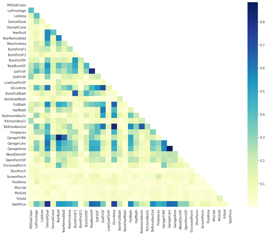
We notice that there are many darkblue-colored squares: there are obvious correlations such as between the number of rooms at each level and the surface of that level (ground or higher floors), between surfaces of different levels, and also between surface and capacity of garages.
These columns give almost the same information, so we can get rit of extra ones.
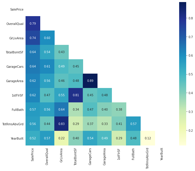
We can also look to features that are directly correlated with the 'SalePrice': we get 'GrLivArea', 'TotalBsmtSF', and 'OverallQual'.
# SalePrice correlation matrix
n = 10
cols = corrmat.nlargest(n, 'SalePrice')['SalePrice'].index # List of highly correlated colums with 'SalePrice'
cm = np.corrcoef(pd.concat([df_train, df_train_target], axis=1)[cols].values.T)
mask = np.zeros_like(cm)
mask[np.triu_indices_from(cm)] = True
with sns.axes_style("white"):
    f, ax = plt.subplots(figsize=(12, 9))
    ax = sns.heatmap(cm,
                     mask=mask,
                     cbar=True,
                     annot=True,
                     square=True,
                     fmt='.2f',
                     annot_kws={'size': 10},
                     yticklabels=cols.values,
                     xticklabels=cols.values,
                     cmap="YlGnBu")
    plt.show()
Scatter Plot
sns.set()
cols = ['SalePrice', 'OverallQual', 'GrLivArea', 'TotalBsmtSF', '1stFlrSF', 'TotRmsAbvGrd', 'YearBuilt', 'GarageYrBlt', 'GarageCars', 'GarageArea']
sns.pairplot(pd.concat([df_train, df_train_target], axis=1)[cols], size = 2.5)
plt.show();
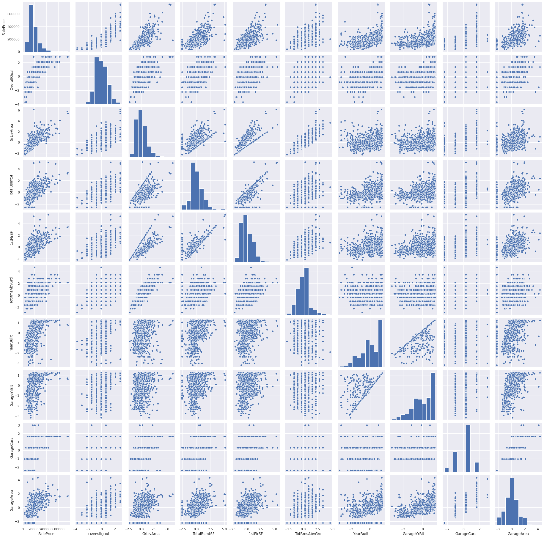
we can see an exponential relation between sale price and build year especially during the recent year.
Garage build year and build year are related but not always equal.
Garage capacity is a result of its area.
# Numerical columns to keep
numerical_cols = ['GrLivArea',
                  'TotalBsmtSF',
                  'OverallQual',
                  'TotalBsmtSF',
                  'GrLivArea',
                  'YearBuilt',
                  'GarageArea',
                  'FullBath',
                  'MSSubClass',
                  'YearRemodAdd']
df_train_num = df_train[numerical_cols]
df_test_num = df_test[numerical_cols]
print("Training data:", df_train_num.shape)
print("Testing data:", df_test_num.shape)
Training data: (1200, 10)
Testing data: (260, 10)
df_num = pd.concat([df_train_num, df_test_num], ignore_index=True)
Non-Numerical/Categorical Fields
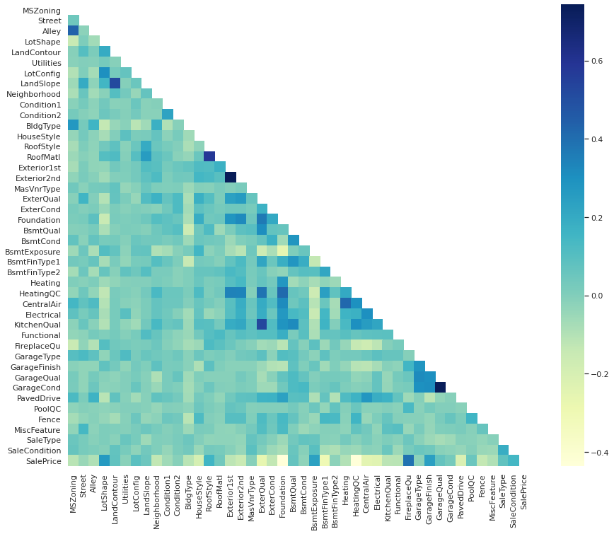
The first step is to find eventual correlations between these fields and if there are interesting relations with ‘SalePrice’ target.
Then, we will convert them to numerical fields using the One-Hot-Encoding and the Label Encoding methods. This step is very important in order to be able to train our model later.
Label Encoding will be used for fields with comparable values, e.g. ‘GarageQual’ whose values can be converted to 5, 4, 3, 2, 1 and 0 for Ex (Excellent), Gd (Good), TA (Typical/Average), Fa (Fair), Po (Poor) and NA (No Garage) respectively.
One-Hot-Encoding will be used for other categorical fields whose values are not comparable, e.g. ‘MSZoning’ for zone classification.
# Print fields' types
df_train.dtypes.unique()
array([dtype('float64'), dtype('O')], dtype=object)
# Extracting non-nemeric fields
df_train_non_num = df_train.select_dtypes(include=['O'])
df_train_non_num.head()
| MSZoning | Street | Alley | LotShape | LandContour | Utilities | LotConfig | LandSlope | Neighborhood | Condition1 | ... | GarageType | GarageFinish | GarageQual | GarageCond | PavedDrive | PoolQC | Fence | MiscFeature | SaleType | SaleCondition | |
|---|---|---|---|---|---|---|---|---|---|---|---|---|---|---|---|---|---|---|---|---|---|
| 0 | RL | Pave | NaN | Reg | Lvl | AllPub | Inside | Gtl | CollgCr | Norm | ... | Attchd | RFn | TA | TA | Y | NaN | NaN | NaN | WD | Normal |
| 1 | RL | Pave | NaN | Reg | Lvl | AllPub | FR2 | Gtl | Veenker | Feedr | ... | Attchd | RFn | TA | TA | Y | NaN | NaN | NaN | WD | Normal |
| 2 | RL | Pave | NaN | IR1 | Lvl | AllPub | Inside | Gtl | CollgCr | Norm | ... | Attchd | RFn | TA | TA | Y | NaN | NaN | NaN | WD | Normal |
| 3 | RL | Pave | NaN | IR1 | Lvl | AllPub | Corner | Gtl | Crawfor | Norm | ... | Detchd | Unf | TA | TA | Y | NaN | NaN | NaN | WD | Abnorml |
| 4 | RL | Pave | NaN | IR1 | Lvl | AllPub | FR2 | Gtl | NoRidge | Norm | ... | Attchd | RFn | TA | TA | Y | NaN | NaN | NaN | WD | Normal |
5 rows × 43 columns
df_train_non_num.nunique()
MSZoning          5
Street            2
Alley             2
LotShape          4
LandContour       4
Utilities         2
LotConfig         5
LandSlope         3
Neighborhood     25
Condition1        9
Condition2        7
BldgType          5
HouseStyle        8
RoofStyle         5
RoofMatl          6
Exterior1st      14
Exterior2nd      15
MasVnrType        4
ExterQual         4
ExterCond         5
Foundation        6
BsmtQual          4
BsmtCond          4
BsmtExposure      4
BsmtFinType1      6
BsmtFinType2      6
Heating           4
HeatingQC         5
CentralAir        2
Electrical        5
KitchenQual       4
Functional        7
FireplaceQu       5
GarageType        6
GarageFinish      3
GarageQual        5
GarageCond        5
PavedDrive        3
PoolQC            3
Fence             4
MiscFeature       3
SaleType          9
SaleCondition     6
dtype: int64
non_num_corr = pd.concat([df_train_non_num.apply(lambda x: x.factorize()[0]), df_train_target], axis=1).corr()
mask = np.zeros_like(non_num_corr)
mask[np.triu_indices_from(mask)] = True
with sns.axes_style("white"):
    f, ax = plt.subplots(figsize=(16, 12))
    ax = sns.heatmap(non_num_corr, mask=mask, square=True, cmap="YlGnBu")
# columns to convert to numerical values
label_encoding_cols = ['Utilities',
                'LandSlope',
                'ExterQual',
                'ExterCond',
                'BsmtQual',
                'BsmtCond',
                'BsmtExposure',
                'BsmtFinType1',
                'BsmtFinType2',
                'HeatingQC',
                'CentralAir',
                'KitchenQual',
                'Functional',
                'FireplaceQu',
                'GarageType',
                'GarageFinish',
                'GarageQual',
                'GarageCond',
                'PavedDrive',
                'PoolQC',
                'Fence']
one_hot_cols = ['MSZoning',
                       'Street',
                       'Alley',
                       'LotShape',
                       'LandContour',
                       'LotConfig',
                       'Neighborhood',
                       'Condition1',
                       'Condition2',
                       'BldgType',
                       'HouseStyle',
                       'RoofStyle',
                       'RoofMatl',
                       'Exterior1st',
                       'Exterior2nd',
                       'MasVnrType',
                       'Foundation',
                       'Heating',
                       'Electrical',
                       'MiscFeature',
                       'SaleType',
                       'SaleCondition']
all_data = pd.concat([df_train, df_test], ignore_index=True)
all_data.shape
(1460, 79)
# Convert categorical variable into indicator variables
df_cat_one_hot = pd.get_dummies(all_data[one_hot_cols], dummy_na=True, columns=one_hot_cols, drop_first=True)
df_cat_one_hot.shape
(1460, 162)
from sklearn.preprocessing import LabelEncoder, OneHotEncoder
df_label_encoding = pd.DataFrame(columns=label_encoding_cols)
for col in label_encoding_cols:
  labelencoder = LabelEncoder()
  df_label_encoding[col] = labelencoder.fit_transform(all_data[col].astype(str))
  # print(labelencoder.fit_transform(df_train[col].astype(str)))
df_label_encoding.head()
| Utilities | LandSlope | ExterQual | ExterCond | BsmtQual | BsmtCond | BsmtExposure | BsmtFinType1 | BsmtFinType2 | HeatingQC | ... | KitchenQual | Functional | FireplaceQu | GarageType | GarageFinish | GarageQual | GarageCond | PavedDrive | PoolQC | Fence | |
|---|---|---|---|---|---|---|---|---|---|---|---|---|---|---|---|---|---|---|---|---|---|
| 0 | 0 | 0 | 2 | 4 | 2 | 3 | 3 | 2 | 5 | 0 | ... | 2 | 6 | 5 | 1 | 1 | 4 | 4 | 2 | 3 | 4 |
| 1 | 0 | 0 | 3 | 4 | 2 | 3 | 1 | 0 | 5 | 0 | ... | 3 | 6 | 4 | 1 | 1 | 4 | 4 | 2 | 3 | 4 |
| 2 | 0 | 0 | 2 | 4 | 2 | 3 | 2 | 2 | 5 | 0 | ... | 2 | 6 | 4 | 1 | 1 | 4 | 4 | 2 | 3 | 4 |
| 3 | 0 | 0 | 3 | 4 | 3 | 1 | 3 | 0 | 5 | 2 | ... | 2 | 6 | 2 | 5 | 2 | 4 | 4 | 2 | 3 | 4 |
| 4 | 0 | 0 | 2 | 4 | 2 | 3 | 0 | 2 | 5 | 0 | ... | 2 | 6 | 4 | 1 | 1 | 4 | 4 | 2 | 3 | 4 |
5 rows × 21 columns
Missing Data
# Missing Data
total = df_train.isnull().sum().sort_values(ascending=False)
percent = (df_train.isnull().sum()/df_train.isnull().count()).sort_values(ascending=False)
missing_data = pd.concat([total, percent], axis=1, keys=['Total', 'Percent'])
missing_data.head(20)
| Total | Percent | |
|---|---|---|
| PoolQC | 1196 | 0.996667 |
| MiscFeature | 1153 | 0.960833 |
| Alley | 1125 | 0.937500 |
| Fence | 973 | 0.810833 |
| FireplaceQu | 564 | 0.470000 |
| LotFrontage | 210 | 0.175000 |
| GarageType | 67 | 0.055833 |
| GarageFinish | 67 | 0.055833 |
| GarageQual | 67 | 0.055833 |
| GarageCond | 67 | 0.055833 |
| GarageYrBlt | 67 | 0.055833 |
| BsmtExposure | 33 | 0.027500 |
| BsmtFinType2 | 33 | 0.027500 |
| BsmtCond | 32 | 0.026667 |
| BsmtFinType1 | 32 | 0.026667 |
| BsmtQual | 32 | 0.026667 |
| MasVnrArea | 6 | 0.005000 |
| MasVnrType | 6 | 0.005000 |
| RoofStyle | 0 | 0.000000 |
| RoofMatl | 0 | 0.000000 |
So we will keep the missing values for these columns because they give us information about the house features.
df_train['LotFrontage'].unique()
array([-2.14617436e-01,  4.18239777e-01, -8.80459934e-02, -4.25569840e-01,
        5.87001701e-01,  6.29192182e-01,  2.07287373e-01,             nan,
       -8.05284168e-01, -8.47474649e-01, -3.66503167e-03,  8.82335067e-01,
        8.07159301e-02, -1.72426955e-01,  1.30423988e+00, -5.52141283e-01,
       -1.10061753e+00,  1.68395420e+00,  1.17766843e+00, -9.74046092e-01,
        1.59957324e+00,  1.76833517e+00,  1.65096892e-01,  1.89490661e+00,
       -3.83379360e-01, -9.31855611e-01, -1.56471282e+00, -7.63093687e-01,
        1.26204939e+00, -1.94442715e+00,  7.97954105e-01, -2.98998398e-01,
        2.49477854e-01,  4.60430258e-01,  1.05109699e+00, -4.58555126e-02,
       -2.07099859e+00, -1.60690331e+00,  3.33858815e-01,  2.14804949e+00,
        2.19023997e+00, -1.26937946e+00,  1.47300180e+00,  1.22906411e-01,
        2.91668334e-01, -2.56807917e-01,  1.00890651e+00, -1.52252234e+00,
        8.40144586e-01, -6.36522245e-01,  7.55763624e-01,  5.02620739e-01,
        3.85254492e-02,  2.10585901e+00,  1.55738276e+00,  9.24525548e-01,
        2.69652574e+00, -3.41188879e-01,  6.71382662e-01,  2.99185911e+00,
        1.13547795e+00, -6.78712726e-01, -1.22718898e+00,  3.76049296e-01,
        4.38414498e+00,  1.21985891e+00, -1.30236474e-01,  5.44811220e-01,
       -1.14280802e+00,  1.38862084e+00,  9.66716029e-01, -1.69128427e+00,
        2.48557334e+00,  2.94966863e+00, -1.48033186e+00, -1.39595090e+00,
        2.02147805e+00,  7.13573143e-01,  1.93709709e+00,  3.37157344e+00,
        1.72614468e+00, -8.89665130e-01,  1.09328747e+00, -4.67760321e-01,
       -1.43814138e+00, -5.94331764e-01,  1.34643036e+00, -5.09950802e-01,
       -1.35376042e+00,  1.64176372e+00,  2.52776382e+00, -7.20903207e-01,
        2.82309719e+00, -1.05842705e+00,  1.51519228e+00,  1.43081132e+00,
       -1.18499850e+00, -1.31156994e+00,  3.11843055e+00,  1.85271613e+00,
        2.44338286e+00,  3.32938296e+00,  1.02486218e+01,  4.13100209e+00,
        4.72166883e+00,  2.86528767e+00,  3.79347825e+00])
The missing data for Garage features won’t affect our work (about 5% of missing data). But we can get rid of Garage and Basement features and only keep the surface because they are not relevent when buying a house.
Finally, we can consider that the masonry veneer features are not essential and have no direct effect on the sale price (‘MasVnrArea’ is correlated with ‘GrLivArea’ and ‘TotRmsAbvGrd’ which are considered as main features).
# fianl df after selecting necessary features
df_final = pd.concat([df_num, df_cat_one_hot, df_label_encoding], axis=1)
df_final.shape
(1460, 193)
# Extract training and testing data
df_train = df_final.iloc[:1200]
df_test = df_final.iloc[1200:]
from scipy import stats
from sklearn import preprocessing
X_train, y_train = df_train.values, df_train_target.values
X_test, y_test = df_test.values, df_test_target.values
Data Labels
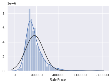
print("Skewness: %f" % df_train_target.skew())
sns.distplot(df_train_target, fit=stats.norm)
Skewness: 1.967215


<matplotlib.axes._subplots.AxesSubplot at 0x7f9d6e95af40>
print("Skewness: %f" % np.log(df_train_target).skew())
sns.distplot(np.log(df_train_target), fit=stats.norm)
Skewness: 0.132714


<matplotlib.axes._subplots.AxesSubplot at 0x7f9d6e82a700>
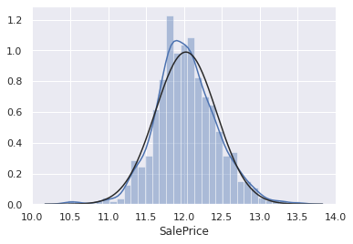
When making predictions, we have to reverse the log transformation (i.e. apply exp transformation) in order to get the ‘SalePrice’. Or we can choose to transform the target label of the testing data.
#Applying log transformation
y_train = np.log(y_train)
y_test = np.log(y_test)
Prediction Model
from sklearn.linear_model import ElasticNet, Lasso,  BayesianRidge, LassoLarsIC
from sklearn.ensemble import RandomForestRegressor,  GradientBoostingRegressor
from sklearn.kernel_ridge import KernelRidge
from sklearn.pipeline import make_pipeline
from sklearn.preprocessing import RobustScaler
from sklearn.base import BaseEstimator, TransformerMixin, RegressorMixin, clone
from sklearn.model_selection import KFold, cross_val_score, train_test_split
from sklearn.metrics import mean_squared_error
import xgboost as xgb
import lightgbm as lgb
import numpy as np
import sklearn.datasets
import sklearn.metrics
from sklearn.model_selection import train_test_split
import tensorflow
import tensorflow.keras as keras
from tensorflow.keras.models import Sequential
from tensorflow.keras.layers import Dense
import optuna
# Define validation function
n_folds = 5

def rmsle_cv(model):
    kf = KFold(n_folds, shuffle=True, random_state=42).get_n_splits(X_train)
    rmse = np.sqrt(-cross_val_score(model, X_train, y_train, scoring="neg_mean_squared_error", cv = kf))
    score = np.mean(rmse)
    return(score)

def rmsle(y, y_pred):
    return np.sqrt(mean_squared_error(y, y_pred))
ENet = make_pipeline(RobustScaler(), ElasticNet(alpha=0.0005, l1_ratio=.9, random_state=3))
score = rmsle_cv(ENet)
print("Enet score is :", score)
Enet score is : 0.13682678960721764
KRR = KernelRidge(alpha=0.6, kernel='polynomial', degree=2, coef0=2.5)

score = rmsle_cv(KRR)
print("KRR score is :", score)
KRR score is : 0.13723828381390502
lasso = make_pipeline(RobustScaler(), Lasso(alpha =0.0005, random_state=1))
score = rmsle_cv(lasso)
print("Lasso score:", score)
Lasso score: 0.13675368241324085
LightGBM + Optuna For Hyperparameters Optimization
It seeks the directions (parameters) that have the biggest impact on the loss of our model and follows this direction for choosing the hyperparameter for the next round.
Just give it the hyperparameters you want to update, how you want to sample from those (uniform / log uniform..) and an evaluation metric (score) and it will work on minimizing it for you.
dtrain = lgb.Dataset(X_train,label=y_train)
dtest = lgb.Dataset(X_test,label=y_test)


def objective(trial):


    param = {
        #"objective": "regression",
        ## "verbosity": -1,
        #"device":"gpu",
        "boostingtype":"goss",
        "learning_rate":trial.suggest_loguniform("learning_rate",0.01,0.1),
        'subsample': trial.suggest_uniform("subsample",0.5,1),
        'feature_fraction':trial.suggest_uniform("subsample",0.5,1),
        "num_leaves": int(trial.suggest_discrete_uniform("num_leaves", 2, 10,1)),
        "n_estimators":int(trial.suggest_loguniform("n_estimators",300,1500)),
        "min_data_in_leaf": int(trial.suggest_loguniform("min_data_in_leaf",4,40)),

    }

    # Add a callback for pruning.
    pruning_callback = optuna.integration.LightGBMPruningCallback(trial, "root_mean_squared_error")

    model = lgb.LGBMRegressor(**param)
    pipe = make_pipeline(RobustScaler(),model)

    score = rmsle_cv(pipe)
    print("Score is", score)
    return score


if __name__ == "__main__":
    study = optuna.create_study(
        pruner=optuna.pruners.MedianPruner(n_warmup_steps=200), direction="minimize")

    study.optimize(objective, n_trials=10)

    print("Number of finished trials: {}".format(len(study.trials)))

    print("Best trial:")
    best_trial = study.best_trial

    print("  Value: {}".format(best_trial.value))

    print("  Params: ")
    for key, value in best_trial.params.items():
        print("    {}: {}".format(key, value))
Score is 0.13600313032409703


[I 2020-05-13 00:02:26,245] Finished trial#0 with value: 0.13600313032409703 with parameters: {'learning_rate': 0.01923119462002535, 'subsample': 0.6626468518675733, 'num_leaves': 9.0, 'n_estimators': 647.6352032192165, 'min_data_in_leaf': 21.033077119746185}. Best is trial#0 with value: 0.13600313032409703.


Score is 0.13640568127865232


[I 2020-05-13 00:02:27,995] Finished trial#1 with value: 0.13640568127865232 with parameters: {'learning_rate': 0.024613463875544094, 'subsample': 0.8507784648943293, 'num_leaves': 10.0, 'n_estimators': 493.03789482908246, 'min_data_in_leaf': 14.362849260435436}. Best is trial#0 with value: 0.13600313032409703.


Score is 0.1349189391273471


[I 2020-05-13 00:02:28,664] Finished trial#2 with value: 0.1349189391273471 with parameters: {'learning_rate': 0.059348839250226805, 'subsample': 0.9945366417050793, 'num_leaves': 3.0, 'n_estimators': 390.90546012907805, 'min_data_in_leaf': 9.898292162804019}. Best is trial#2 with value: 0.1349189391273471.


Score is 0.13871747406835083


[I 2020-05-13 00:02:30,442] Finished trial#3 with value: 0.13871747406835083 with parameters: {'learning_rate': 0.069324825051667, 'subsample': 0.7523892885875515, 'num_leaves': 7.0, 'n_estimators': 1014.0907893209081, 'min_data_in_leaf': 8.00434817044987}. Best is trial#2 with value: 0.1349189391273471.


Score is 0.138256553664015


[I 2020-05-13 00:02:31,248] Finished trial#4 with value: 0.138256553664015 with parameters: {'learning_rate': 0.018382734588964663, 'subsample': 0.7498495471593678, 'num_leaves': 4.0, 'n_estimators': 414.69291940907084, 'min_data_in_leaf': 6.168345054282901}. Best is trial#2 with value: 0.1349189391273471.


Score is 0.14428494968450611


[I 2020-05-13 00:02:31,859] Finished trial#5 with value: 0.14428494968450611 with parameters: {'learning_rate': 0.056910426348052066, 'subsample': 0.8949690215207301, 'num_leaves': 2.0, 'n_estimators': 455.8345176759971, 'min_data_in_leaf': 38.51505322114788}. Best is trial#2 with value: 0.1349189391273471.


Score is 0.13541023518338582


[I 2020-05-13 00:02:33,110] Finished trial#6 with value: 0.13541023518338582 with parameters: {'learning_rate': 0.010969369772362703, 'subsample': 0.6904482246527368, 'num_leaves': 4.0, 'n_estimators': 960.8874925988346, 'min_data_in_leaf': 19.22499177034413}. Best is trial#2 with value: 0.1349189391273471.


Score is 0.13210578425376807


[I 2020-05-13 00:02:34,644] Finished trial#7 with value: 0.13210578425376807 with parameters: {'learning_rate': 0.02184369730127071, 'subsample': 0.5128444945002342, 'num_leaves': 5.0, 'n_estimators': 1187.1548228495471, 'min_data_in_leaf': 15.979845843774275}. Best is trial#7 with value: 0.13210578425376807.


Score is 0.1682655819291983


[I 2020-05-13 00:02:35,218] Finished trial#8 with value: 0.1682655819291983 with parameters: {'learning_rate': 0.017935162873548946, 'subsample': 0.5229929455018336, 'num_leaves': 2.0, 'n_estimators': 357.96774663786687, 'min_data_in_leaf': 13.255524740231005}. Best is trial#7 with value: 0.13210578425376807.


Score is 0.1362679938439728


[I 2020-05-13 00:02:36,435] Finished trial#9 with value: 0.1362679938439728 with parameters: {'learning_rate': 0.016582307774637164, 'subsample': 0.8659955203836165, 'num_leaves': 3.0, 'n_estimators': 1017.6045021394999, 'min_data_in_leaf': 5.488615281157206}. Best is trial#7 with value: 0.13210578425376807.


Number of finished trials: 10
Best trial:
  Value: 0.13210578425376807
  Params:
    learning_rate: 0.02184369730127071
    subsample: 0.5128444945002342
    num_leaves: 5.0
    n_estimators: 1187.1548228495471
    min_data_in_leaf: 15.979845843774275
params = {}
for key, value in best_trial.params.items():
  if value > 1:
    params[key] = int(value)
  else :
    params[key] = value

## Little trick to have better accuracy : Divide the learning rate and double the number of learners by same constant (doesn't work here :'( )

params["learning_rate"] *= 0.5
params["n_estimators"] *= 2

GBM = make_pipeline(RobustScaler(), lgb.LGBMRegressor(**params))
rmsle_cv(GBM)
0.13391835487283882
Stacking Models For Predictions
The procedure, for the training part, may be described as follows:
- Split the total training set into two disjoint sets (here train and .holdout)
- Train several base models on the first part (train)
- Test these base models on the second part (holdout)
Use the predictions from 3) (called out-of-folds predictions) as the inputs, and the correct responses (target variable) as the outputs to train a higher level learner called meta-model.
The first three steps are done iteratively . If we take for example a 5-fold stacking , we first split the training data into 5 folds. Then we will do 5 iterations. In each iteration, we train every base model on 4 folds and predict on the remaining fold (holdout fold).
So, we will be sure, after 5 iterations , that the entire data is used to get out-of-folds predictions that we will then use as new feature to train our meta-model in the step 4.
For the prediction part , We average the predictions of all base models on the test data and used them as meta-features on which, the final prediction is done with the meta-model.
class MetaModel(BaseEstimator, RegressorMixin, TransformerMixin):
    def __init__(self, base_models, meta_model, n_folds=5):
        self.base_models = base_models
        self.meta_model = meta_model
        self.n_folds = n_folds

    # We again fit the data on clones of the original models
    def fit(self, X, y):
        self.base_models_ = [list() for x in self.base_models]
        self.meta_model_ = clone(self.meta_model)
        kfold = KFold(n_splits=self.n_folds, shuffle=True, random_state=156)

        # Train cloned base models then create out-of-fold predictions
        # that are needed to train the cloned meta-model
        out_of_fold_predictions = np.zeros((X.shape[0], len(self.base_models)))
        for i, model in enumerate(self.base_models):
            for train_index, holdout_index in kfold.split(X, y):
                instance = clone(model)
                self.base_models_[i].append(instance)
                instance.fit(X[train_index], y[train_index])
                y_pred = instance.predict(X[holdout_index])
                out_of_fold_predictions[holdout_index, i] = y_pred

        # Now train the cloned  meta-model using the out-of-fold predictions as new feature
        self.meta_model_.fit(out_of_fold_predictions, y)
        return self


        #Do the predictions of all base models on the test data and use the averaged predictions as
    #meta-features for the final prediction which is done by the meta-model
    def predict(self, X):
        meta_features = np.column_stack([
            np.column_stack([model.predict(X) for model in base_models]).mean(axis=1)
            for base_models in self.base_models_])
        return self.meta_model_.predict(meta_features)
meta = MetaModel(base_models = (ENet, GBM, KRR), meta_model = lasso)

score = rmsle_cv(meta)
print("Score is ", score)
Score is 0.13132544460806347
meta.fit(X_train, y_train)
meta.base_models_
pred = meta.predict(X_test)
rmsle(pred, y_test)
0.15162988008351325
Deep Learning Model
For this model we used the NovoGrad Optimizer which usesgradient descent method with layer-wise gradient normalization and decoupled weight decay adapted from this paper.
We wrap the optimizer in the lookahead wrapper, the algorithm chooses a search direction by looking ahead at the sequence of K fast weights generated by another optimizer.
We use an exponentially decreasing cyclical learning rate scheduler . Instead of monotonically decreasing the learning rate, this method lets the learning rate cyclically vary between reasonable boundary values.
We train the model using leaky ReLU activation and minimal dropout at the beginning of the net. Batchnormalisation to make loss function smoother. We also use early stopping with a patience of 200 epochs as we suppose that the model generalizes better at earlier stages of training as it didn’t overfit training set yet.
All these addons allow us to train a decent DNN with minimal hyperparameter tuning especially for learning rate.
import tensorflow_addons as tfa
from tensorflow.keras.layers import Dropout , BatchNormalization
from tensorflow.nn import leaky_relu
from tensorflow.keras import backend as K
from tensorflow_addons.optimizers.novograd import NovoGrad
model = Sequential()
n_cols = X_train.shape[1]
print("N_cols=",n_cols)
def rmse(y_true, y_pred):
return K.sqrt(K.mean(K.square(y_pred - y_true)))
def LR(x):
return leaky_relu(x, alpha=0.1)
model.add(Dense(600, activation=LR, input_shape= (n_cols,)))
model.add(BatchNormalization())
model.add(Dropout(0.15))
model.add(Dense(400, activation=LR))
model.add(BatchNormalization())
model.add(Dropout(0.1))
model.add(Dense(300, activation=LR))
model.add(BatchNormalization())
model.add(Dropout(0.1))
model.add(Dense(300, activation=LR))
model.add(BatchNormalization())
model.add(Dense(200, activation=LR))
model.add(BatchNormalization())
model.add(Dense(150, activation=LR))
model.add(BatchNormalization())
model.add(Dense(1))
# Learning rate :
lr_schedule = tfa.optimizers.ExponentialCyclicalLearningRate(
initial_learning_rate=1e-4,
maximal_learning_rate=1e-2,
step_size=2000,
scale_mode="cycle",
gamma=0.96,
name="MyCyclicScheduler")
# Optimizer
opt = NovoGrad(learning_rate=lr_schedule)
opt = tfa.optimizers.Lookahead(opt) ##WRAP OPTIMIZER WITH LookAhead layer
##Early stopping
es = tensorflow.keras.callbacks.EarlyStopping(monitor='val_loss',restore_best_weights=True, patience=200)
model.compile(optimizer=opt, loss=rmse)
# train model
history = model.fit(X_train, y_train, verbose=0, batch_size=40, validation_split=0.2, epochs=1000, callbacks=[es])
# list all data in history
print(history.history.keys())
# summarize history for loss
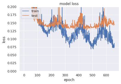
plt.ylim([0,0.2])
plt.plot(history.history['loss'])
plt.plot(history.history['val_loss'])
plt.title('model loss')
plt.ylabel('loss')
plt.xlabel('epoch')
plt.legend(['train', 'test'], loc='upper left')
plt.show()
N_cols= 193
WARNING:tensorflow:From /home/mokhles/.local/lib/python3.8/site-packages/tensorflow/python/ops/resource_variable_ops.py:1813: calling BaseResourceVariable.__init__ (from tensorflow.python.ops.resource_variable_ops) with constraint is deprecated and will be removed in a future version.
Instructions for updating:
If using Keras pass *_constraint arguments to layers.
dict_keys(['loss', 'val_loss'])
y_pred = model.predict(X_test)
rmsle(y_pred, y_test)
0.13674783660080644
Conclusion
We conclude that a good DNN can beat a fine tuned MetaModel on this task.
DNN can deal better with categorical data with low cardinality than any other simple model.
In contrast to LGBM it can map complex interactions between features.
Mokhles Bouzaien
Master of Science in Engineering Student
A self-motivated graduate student in Engineering at IMT Atlantique.