Gradient Descent: Implementation and Visualization
 Gradient descent path
In this notebook, I’ll try to implement the gradient descent algorithm, test it with few predefined functions and visualize its behabiour in order to coclude with the importance of each parameter of the algorithm.
At the end, I will apply the gradient descent algorithm to minimize the mean squared error funcion of the least squares method.
# Imports

%matplotlib inline
import numpy as np
import matplotlib.pyplot as plt
from mpl_toolkits.mplot3d import Axes3D
from matplotlib import cm
# Test Funcions (inspired from https://en.wikipedia.org/wiki/Gradient_descent and http://www.numerical-tours.com/matlab/optim_1_gradient_descent/)

f = lambda x,y : (x-2)**2*(np.sin(y-1))**2+x**2+y**2
g = lambda x,y : (1-x)**2+100*(y-x**2)**2
h = lambda x,y : ( x**2 + 10*y**2 ) / 2
# The partial derivatives

df = lambda x,y : np.array([2*x+2*(x-2)*(np.sin(y-1))**2, 2*y+(x-2)**2*np.sin(2*(y-1))])
dg = lambda x,y : np.array([2*(200*x**3-200*x*y+x-1), 200*(y-x**2)])
dh = lambda x,y : np.array([x,10*y])
# Gradient descent

def grad(fun=h,                              # The function to minimize
         dfun=dh,                            # The partial derivatives
         init=np.array([1.5,1.5]),           # Starting point
         gamma=0.5,                          # Gradient step
         precision=0.01,                     # Precision
         max_iters=1000,                     # Maximum number of iterations
         xlim=(-2, 2),                       # X limits (for graphic representation)
         ylim=(-2, 2),                       # Y limits (for graphic representation)
         arrows=False,                       # Plot steps
         e=0.005):                           # Meshgrid stepsize (for graphic representation)

    X = np.arange(xlim[0],xlim[1], e)
    Y = np.arange(ylim[0],ylim[1], e)
    X, Y = np.meshgrid(X, Y)
    Z = fun(X, Y)
    cur_a = init

    fig = plt.figure(figsize=(16,8))
    # Representing the 3-D function
    ax = plt.subplot(121, projection = '3d')
    ax.plot_surface(X, Y, Z, cmap = cm.coolwarm, linewidth = 0, antialiased = False)
    ax.contour(X, Y, Z, zdir = 'z', offset = -0.8, cmap = cm.coolwarm)
    ax.set_title('f function graph', fontsize = 15)
    ax.set_xlabel('x')
    ax.set_ylabel('y')
    ax.set_zlabel('z')
    # Representing contours and the starting point
    ax = plt.subplot(122)
    plt.imshow(Z, extent = (xlim[0],xlim[1],ylim[0],ylim[1]), cmap=cm.coolwarm, origin = 'lower')
    plt.contour(X, Y, Z, 30)
    plt.plot(cur_a[0], cur_a[1], 'o', color='r')


    previous_step_size = 1 # To enter while loop
    iters = 0 # Iteration counter
    #print(previous_step_size > precision and iters < max_iters)

    while previous_step_size > precision and iters < max_iters:
        prev_a = cur_a
        cur_a = cur_a - gamma * dfun(prev_a[0], prev_a[1])
        previous_step_size = np.linalg.norm(cur_a - prev_a)
        if arrows:
            dx, dy = cur_a[0] - prev_a[0], cur_a[1] - prev_a[1]
            plt.arrow(prev_a[0], prev_a[1], dx, dy, length_includes_head=True, head_width=0.02)
        plt.plot(cur_a[0], cur_a[1], '.',color='k')
        iters += 1
    print("The final solution is ",cur_a)
    print('We obtain the solution with a '+str(precision)+' precision, after '+str(iters)+' iterations.')
    return cur_a
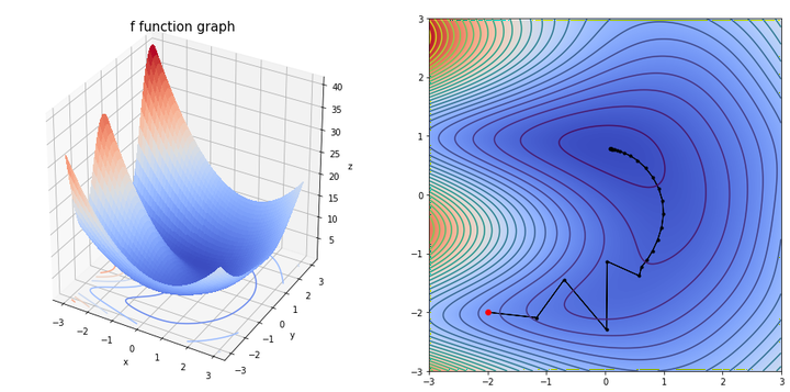
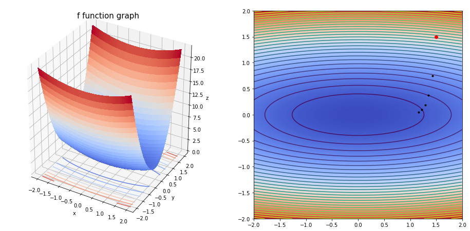
$f(x,y)=(x-2)^2*(sin(y-1))^2+x^2+y^2$
grad(fun=f,
     dfun=df,
     init=np.array([-2,-2]),
     gamma=0.05,
     precision=1e-04,
     max_iters=10000,
     xlim=(-3, 3),
     ylim=(-3, 3))
The final solution is  [0.09269109 0.77872974]
We obtain the solution with a 0.0001 precision, after 155 iterations.


array([0.09269109, 0.77872974])
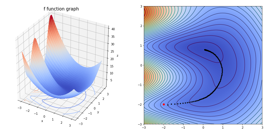
grad(fun=f,
     dfun=df,
     init=np.array([-2,-2]),
     gamma=0.2,
     precision=1e-04,
     max_iters=10000,
     xlim=(-3, 3),
     ylim=(-3, 3),
     arrows=True)
The final solution is  [0.0918675  0.77892566]
We obtain the solution with a 0.0001 precision, after 36 iterations.


array([0.0918675 , 0.77892566])

grad(fun=f,
     dfun=df,
     init=np.array([-2,-2]),
     gamma=0.5,
     precision=1e-03,
     max_iters=100,
     xlim=(-3, 3),
     ylim=(-3, 3),
     arrows=1)
The final solution is  [0.07586343 0.09220978]
We obtain the solution with a 0.001 precision, after 100 iterations.


array([0.07586343, 0.09220978])
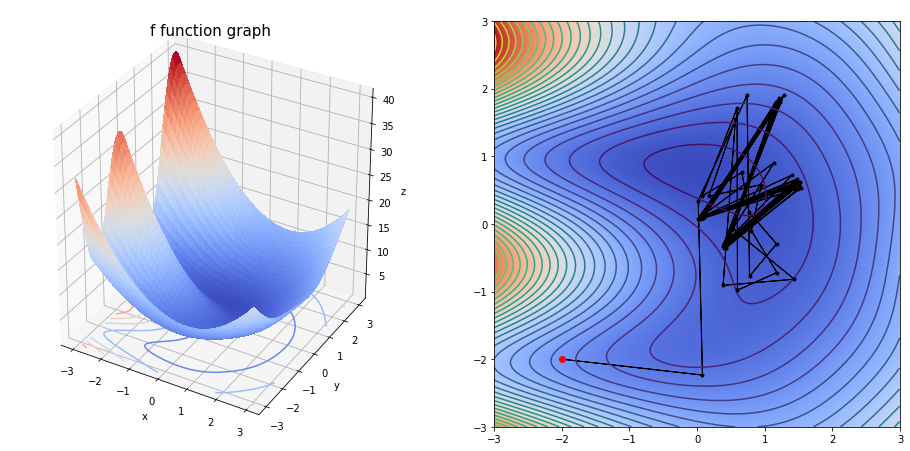
As we can see, if we increase the step size ($\gamma$) from $0.05$ to $0.2$ we can converge to the minimum very fast ($36$ iterations instead of $155$). But after increasing the step size to $0.5$ the algorithm seems not to converge (at least after $10,000$ iterations).
$g(x,y)=(1-x)^2+100*(y-x^2)^2$

grad(fun=g,
     dfun=dg,
     init=np.array([0.5,0.5]),
     gamma=0.005, precision=1e-03,
     max_iters=10000,
     xlim=(0, 2),
     ylim=(0, 2))
The final solution is  [0.46330448 0.2853615 ]
We obtain the solution with a 0.001 precision, after 10000 iterations.


array([0.46330448, 0.2853615 ])

grad(fun=g,
     dfun=dg,
     init=np.array([1.75,1.5]),
     gamma=0.001,
     precision=1e-05,
     max_iters=10000,
     xlim=(0, 2),
     ylim=(0, 2),
     arrows=1)
The final solution is  [1.01127616 1.02272428]
We obtain the solution with a 1e-05 precision, after 8019 iterations.


array([1.01127616, 1.02272428])

grad(fun=g,
     dfun=dg,
     init=np.array([0.7,0.5]),
     gamma=0.001,
     precision=1e-05,
     max_iters=50000,
     xlim=(0, 2),
     ylim=(0, 2))
The final solution is  [0.98892335 0.97792476]
We obtain the solution with a 1e-05 precision, after 7166 iterations.


array([0.98892335, 0.97792476])
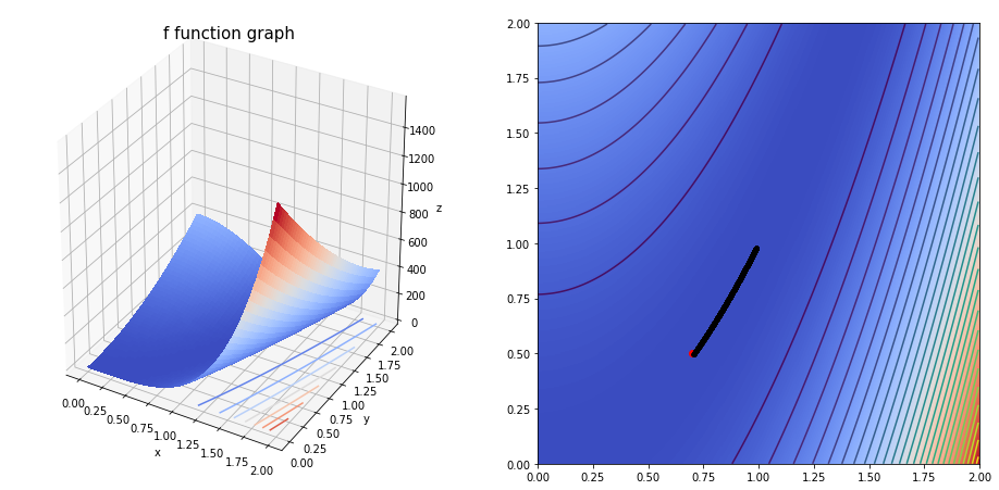
TL;DR The starting point is important to get a convergent algorithm.
$h(x,y)=0.5*( x^2 + 10*y^2 )$
grad(fun=h,
     dfun=dh,
     init=np.array([1.5,1.5]),
     gamma=0.05,
     precision=1e-03,
     max_iters=10000,
     xlim=(-2, 2),
     ylim=(-2, 2),
     arrows=1)
The final solution is  [1.82104767e-02 1.93870456e-26]
We obtain the solution with a 0.001 precision, after 86 iterations.


array([1.82104767e-02, 1.93870456e-26])

grad(fun=h, dfun=dh, init=np.array([1.5,1.5]), gamma=0.05, precision=1e-01, max_iters=10000, xlim=(-2, 2), ylim=(-2, 2))
The final solution is  [1.16067141 0.046875  ]
We obtain the solution with a 0.1 precision, after 5 iterations.


array([1.16067141, 0.046875  ])
Not enough iterations since fastly we reached a point where $||a_{n+1}-a_n||=||-\gamma\nabla h(a_n)||<precision=0.1$.
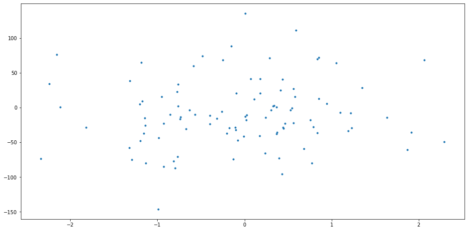
Gradient Descent Algorithm applied to Least Squares Method
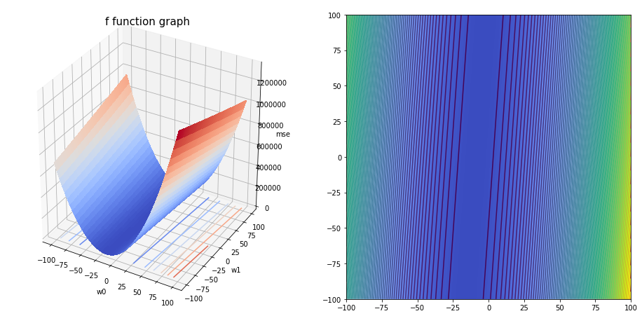
The least squares method consists of minimizing the Mean Squared Error function defined as : $MSE(w_0,w_1)=\frac{1}{N}\sum_{i=1}^{N}{(f(x_i)-y_i)^2}=\frac{1}{N}\sum_{i=1}^{N}{(w_0+w_1x_i-y_i)^2}$
from sklearn.datasets import make_regression
N = 100 # Sample size
# Generating dataset
X, y = make_regression(N, 1, noise=50)
X = np.array([k[0] for k in X])
fig = plt.figure(figsize=(16,8))
plt.scatter(X,y,marker='.')
plt.show()
mse = lambda w0,w1 : (1/N)*np.square(sum(w0+w1*X[i]-y[i] for i in range(N)))
dmse = lambda w0,w1 : np.array([2*w0+(2*w1/N)*sum(X)-(2/N)*sum(y),
                               (2/N)*sum(X[i]*(w0+w1*X[i]-y[i]) for i in range(N))])
Xr = np.arange(-100,100, 0.1)
Yr = np.arange(-100,100, 0.1)
Xr, Yr = np.meshgrid(Xr, Yr)
Zr = mse(Xr, Yr)

fig_1 = plt.figure(figsize=(16,8))
ax = plt.subplot(121, projection = '3d')
ax.plot_surface(Xr, Yr, Zr, cmap = cm.coolwarm, linewidth = 0, antialiased = False)
ax.contour(Xr, Yr, Zr, zdir = 'z', offset = 0, cmap = cm.coolwarm)
ax.set_title('f function graph', fontsize = 15)
ax.set_xlabel('w0')
ax.set_ylabel('w1')
ax.set_zlabel('mse')

ax = plt.subplot(122)
plt.imshow(Zr, extent = (-100,100,-100,100), cmap=cm.coolwarm, origin = 'lower')
plt.contour(Xr, Yr, Zr, 100)
<matplotlib.contour.QuadContourSet at 0x7f8345424710>
w0,w1 = grad(fun=mse,
             dfun=dmse,
             init=np.array([0,-75]),
             gamma=0.05,
             precision=1e-05,
             max_iters=10000,
             xlim=(-100, 100),
             ylim=(-100, 100),
             e=0.1)
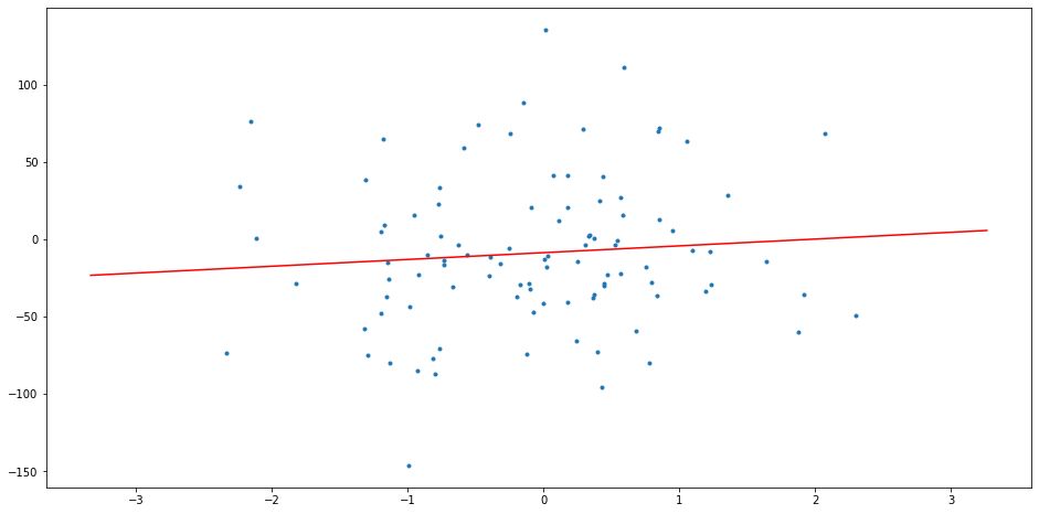
The final solution is  [-8.66316056  4.390188  ]
We obtain the solution with a 1e-05 precision, after 149 iterations.
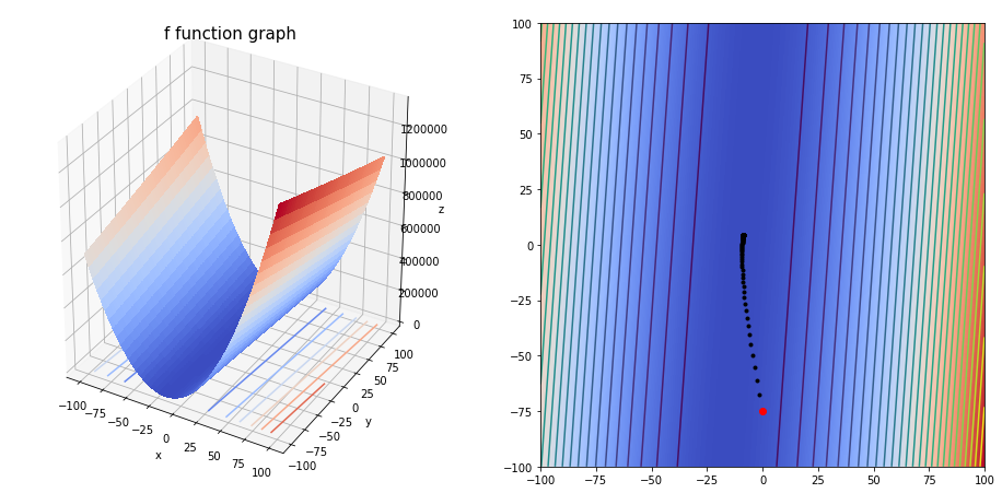
fig_1 = plt.figure(figsize=(16,8))
xrange = np.arange(min(X)-1, max(X)+1, 0.1)
plt.plot(xrange, w0+w1*xrange, color='r')
plt.scatter(X,y,marker='.')
plt.show()
Mokhles Bouzaien
Master of Science in Engineering Student
A self-motivated graduate student in Engineering at IMT Atlantique.